How to Master HVAC Ventilation Calculation: Formulas, Standards, and Practical Tips

The Critical Role of Precision in HVAC Ventilation Design

The integrity of a building’s environmental control system relies entirely on the accuracy of the initial hvac ventilation calculation. Without rigorous mathematical modeling, even the most sophisticated mechanical equipment cannot guarantee indoor air quality (IAQ) or thermal comfort. In engineering terms, ventilation is not merely the movement of air; it is the precise management of differential pressures, volumetric flow rates, and thermal loads to create a safe and compliant atmosphere. A minor miscalculation in airflow requirements can lead to “sick building syndrome,” regulatory non-compliance, and significantly inflated operational costs due to inefficient energy usage.

Mastering these calculations requires a deep understanding of fluid dynamics and the specific requirements of the occupied space. Engineers must look beyond simple square footage to analyze the complex interaction between air distribution networks, such as spiral duct and fittings, and the mechanical force provided by air movers. The objective is to determine the exact Cubic Feet per Minute (CFM) and Air Changes per Hour (ACH) required to dilute contaminants and maintain oxygen levels. This process involves selecting the appropriate air ducts to minimize static pressure loss while ensuring that the velocity of the air does not create noise or draft issues for occupants.

Compliance with industry benchmarks, specifically ASHRAE Standard 62.1, serves as the baseline for these engineering decisions. This standard dictates the minimum ventilation rates necessary to ensure acceptable IAQ, which varies drastically based on occupancy density and building usage. Whether designing for a high-density conference room or a sterile laboratory, the calculation must account for the specific demands placed on tubeaxial commercial fans and other supply equipment. Furthermore, accurate sizing prevents the common pitfall of equipment oversizing, which leads to short-cycling and premature component failure, or undersizing, which results in an inability to meet peak load demands.

To achieve true system optimization, ventilation calculations must also integrate heat load analysis. Understanding sensible and latent heat gains allows designers to refine airflow strategies that handle moisture control and temperature regulation simultaneously. This holistic approach ensures that the supply grille delivers air effectively without bypassing critical zones. For professionals seeking to deepen their technical expertise, understanding how to size air ducts based on these calculations is a prerequisite for success. The following sections will provide a comprehensive technical breakdown of the essential formulas, compliance standards, and strategic methodologies required to execute high-precision ventilation design.

Precise HVAC ventilation calculation is the cornerstone of designing systems that ensure indoor air quality, regulatory compliance, and operational sustainability. The following takeaways outline the essential formulas, standards, and strategic considerations required to execute these calculations with engineering accuracy.

• Precision in fundamental formulas drives system performance: Mastering the calculation of Cubic Feet per Minute (CFM) and Air Changes per Hour (ACH) is essential for ensuring systems strictly meet airflow requirements relative to specific room volumes.
• Adherence to ASHRAE 62.1 ensures compliance and safety: Strictly applying established industry benchmarks guarantees that ventilation rates satisfy legal codes and health standards, mitigating liabilities associated with poor indoor air quality.
• Occupancy loads dictate dynamic ventilation requirements: Accurate calculations must factor in maximum occupancy density and specific space usage to prevent under-ventilation during peak hours or energy waste during low-traffic periods.
• Optimized calculations bridge the gap to energy efficiency: Beyond basic airflow compliance, precise ventilation sizing directly correlates to reduced energy consumption, balancing superior air quality with minimized utility costs.
• Integrating heat load analysis refines sizing precision: Incorporating sensible and latent heat gain data into ventilation formulas prevents system undersizing and ensures adequate moisture control and thermal comfort.
• Building envelope integrity impacts calculation accuracy: Adjusting formulas to account for air leakage, insulation quality, and external environmental factors results in a more realistic and effective HVAC design.
• Demand-controlled ventilation offers adaptive efficiency: Utilizing calculations that allow for variable airflow based on real-time sensors can significantly reduce operational costs without compromising environmental standards.

With these foundational principles established, the subsequent sections will provide a deep dive into the specific mathematical formulas, step-by-step calculation methods, and the detailed application of ASHRAE standards necessary for mastering HVAC ventilation design.

Core Fundamentals of HVAC Ventilation Calculation

Defining the Physics of Airflow

To truly master hvac ventilation calculation, one must first deconstruct the underlying physics that govern air movement within a built environment. Ventilation is not merely the introduction of fresh air; it is the precise management of fluid dynamics to maintain thermodynamic equilibrium and contaminant control. At the heart of every ventilation design lies the continuity equation, a fundamental principle of fluid mechanics stating that mass is conserved as air moves through a duct system.

The primary relationship between volumetric flow rate, velocity, and the cross-sectional area of the conduit is expressed through the following equation:Q = V x A

In this formula, Q represents the airflow volume (typically in Cubic Feet per Minute, or CFM), V denotes the velocity of the air (in Feet per Minute, or FPM), and A is the cross-sectional area of the duct (in Square Feet). Understanding this relationship is critical because it dictates the trade-offs inherent in system design. For a fixed volume of air required to cool a space, reducing the duct size (Area) necessitates a proportional increase in Velocity. While higher velocities allow for smaller ducts, they exponentially increase friction losses and noise generation. Conversely, understanding what is ventilation in HVAC requires recognizing that low-velocity systems, while quieter and more energy-efficient, require significantly larger spatial footprints for ductwork.

Furthermore, this equation serves as the baseline for determining dynamic pressure, which is the kinetic energy component of the total pressure in an airstream. Engineers must balance static pressure (potential energy pushing against duct walls) with velocity pressure (kinetic energy of movement) to ensure air reaches the furthest terminal units without excessive energy expenditure.

Mastering HVAC CFM Calculation Formulas

Once the physics of flow are understood, the engineer must quantify the volume of air required to treat a specific thermal load. This is the cornerstone of system sizing. The hvac cfm calculation connects the thermal requirements of a space (measured in BTUs) with the volumetric flow rate required to remove that heat. For sensible heat—the heat that causes a change in temperature without a change in phase—the governing equation is derived from the specific heat capacity and density of air.

The standard formula used across the industry is:CFM = BTU / (1.08 x ΔT)

Here, BTU represents the sensible heat gain (British Thermal Units per hour), and ΔT (Delta T) is the temperature difference between the supply air and the room design temperature. The constant 1.08 is a derivation of several physical properties of air at standard conditions (sea level, 70°F). It is calculated as:1.08 = 0.075 (lb/ft³ density) x 0.24 (Btu/lb°F specific heat) x 60 (min/hr)

Crucial Engineering Note: The constant 1.08 is accurate only for standard air density. Engineers working at high altitudes or with extreme temperatures must adjust this air density factor. For example, at 5,000 feet of elevation, the air density drops significantly, requiring a higher CFM to transport the same amount of thermal energy. Failing to adjust this constant results in undersized systems that cannot meet the sensible cooling load.

Calculating Air Changes Per Hour (ACH)

While CFM addresses the thermal load, specific environments require ventilation based on volumetric turnover to ensure contaminant dilution. This is measured in Air Changes Per Hour (ACH). This metric is particularly vital in critical environments such as healthcare facilities, laboratories, and cleanrooms, where the removal of airborne pathogens or chemical fumes takes precedence over thermal comfort.

The calculation for ACH is defined as:ACH = (CFM x 60) / Room Volume

To use this formula effectively, the engineer must first calculate the Room Volume (Length x Width x Height). By rearranging the formula, one can determine the required CFM to meet a specific ACH standard:Required CFM = (ACH x Room Volume) / 60

A robust ventilation strategy always involves cross-referencing calculations. The engineer should calculate the CFM required for thermal loads (Sensible Heat) and the CFM required for ACH (Dilution). The system must be sized for whichever value is higher. This ensures that the system not only maintains temperature but also provides adequate air turnover to prevent the buildup of CO2, VOCs, and particulate matter.

Adhering to ASHRAE Standards and Compliance Codes

Navigating ASHRAE Standard 62.1

Compliance with ASHRAE Standard 62.1 is the regulatory bedrock of commercial ventilation design. This standard outlines the “Ventilation Rate Procedure” (VRP), a prescriptive method for determining the minimum outdoor airflow required to maintain acceptable Indoor Air Quality (IAQ). Unlike simple thermal calculations, the VRP acknowledges that ventilation requirements are driven by two distinct factors: the people occupying the space and the building materials themselves.

ASHRAE separates these loads into two coefficients:

• People Outdoor Air Rate (Rp): The amount of fresh air required per person (CFM/person) to dilute bioeffluents and CO2 generated by metabolism.
• Area Outdoor Air Rate (Ra): The amount of fresh air required per square foot (CFM/ft²) to dilute off-gassing from furniture, carpets, paints, and building materials.

This dual-source methodology ensures that even an unoccupied building receives a baseline of ventilation to prevent “sick building syndrome” caused by material off-gassing.

Ventilation Rate Calculation Formula Application

To determine the Breathing Zone Outdoor Airflow (Vbz), engineers must apply the ventilation rate calculation formula specified in the standard. This calculation combines the people-based and area-based requirements into a single value for the specific zone.

The governing equation is:Vbz = (Rp x Pz) + (Ra x Az)

In this equation:

• Rp = Outdoor airflow rate per person (from ASHRAE Table 6.1).
• Pz = Zone Population (the largest number of people expected to occupy the zone during typical usage).
• Ra = Outdoor airflow rate per unit area (from ASHRAE Table 6.1).
• Az = Zone Floor Area (the net occupiable floor area of the zone).

For example, in a modern office space, the Rp might be 5 CFM/person, and the Ra might be 0.06 CFM/ft². If the space is 1,000 sq. ft. with 10 people, the calculation is (5 x 10) + (0.06 x 1000) = 50 + 60 = 110 CFM of outdoor air. This Vbz is the absolute minimum fresh air that must reach the breathing zone (between 3 and 72 inches above the floor).

Safety Factors and Contaminant Control

While ASHRAE Standard 62.1 provides the legal minimums, engineering for high-performance buildings often requires exceeding these baselines. In areas with high concentrations of Volatile Organic Compounds (VOCs) or industrial particulates, the standard VRP may not provide sufficient dilution. Engineers must apply safety factors or utilize the Indoor Air Quality Procedure (IAQP), which uses mass-balance analysis of specific contaminants to determine rates.

Critical Insight: Code compliance is not synonymous with optimal performance. The ASHRAE minimums are designed to satisfy 80% of occupants. To achieve true building health and superior cognitive function for occupants, top-tier engineers often design for 30% above ASHRAE minimums. However, this increase must be balanced against energy consumption, highlighting that accurate calculations are the foundation of building energy efficiency, not just compliance.

Once the breathing zone requirement is established, the engineer must account for the efficiency of the air distribution system, leading us to the nuances of occupancy and zone effectiveness.

Integrating Occupancy and Usage Loads

Dynamic Occupancy Density Calculations

Static calculations often fail to account for the dynamic nature of commercial buildings. Determining Pz (Zone Population) requires an analysis of peak vs. average occupancy. Designing strictly for peak occupancy (e.g., a conference room fully packed) can lead to massive equipment oversizing, resulting in short-cycling and poor humidity control during partial load conditions.

Engineers utilize diversity factors to account for the probability that not every room in a building will be at peak occupancy simultaneously. However, for the ventilation calculation of a specific zone, the peak number is usually required to ensure safety. To manage this variability, Variable Air Volume (VAV) systems are employed. Effective HVAC ventilation design relies on accurately predicting these load profiles to size the central plant appropriately without under-ventilating critical zones during high-traffic periods.

Zone Effectiveness and Air Distribution

Calculating the required airflow is only half the battle; ensuring that air actually reaches the occupants is the other. ASHRAE introduces the Zone Air Distribution Effectiveness (Ez) metric. This coefficient adjusts the required outdoor air intake based on how effectively the supply air mixes with the room air. Poor mixing (short-circuiting) requires the system to bring in more outdoor air to achieve the same result in the breathing zone.

The required outdoor air intake (Roz) is calculated as Roz = Vbz / Ez. Below is a comparison of common distribution strategies and their effectiveness values:

This data highlights that selecting efficient distribution methods, such as displacement ventilation, directly impacts the calculation of required intake air, thereby influencing equipment sizing and energy usage.

Incorporating Heat Load and Thermodynamics

Sensible vs. Latent Heat Gain Impact

A comprehensive air flow calculations hvac strategy must distinguish between sensible heat (temperature) and latent heat (moisture). In humid climates or high-occupancy zones (gyms, auditoriums), the latent load can be significant. The standard CFM formula addresses only sensible heat. To calculate the airflow required to manage humidity, engineers must use the latent heat equation.

The formula for latent airflow requirements is:Latent CFM = BTU_latent / (0.68 x ΔGrains)

In this equation, BTU_latent is the moisture load, and ΔGrains is the difference in humidity ratio (grains of water per pound of dry air) between the room air and the supply air. The constant 0.68 is derived from the latent heat of vaporization of water (approximately 1061 BTU/lb) combined with air density factors (4.5 factor adjusted for grains). If the Latent CFM calculation yields a higher number than the Sensible CFM, the system must be sized based on the latent requirement to prevent mold growth and occupant discomfort. This is often the driving factor in Dedicated Outdoor Air Systems (DOAS).

Psychrometrics in Ventilation Sizing

To accurately determine the properties of the air entering and leaving the coil, engineers utilize psychrometrics—the thermodynamic study of gas-vapor mixtures. Ventilation calculations cannot be performed in a vacuum; the outdoor air (OA) mixes with return air (RA) to form mixed air (MA). The properties of this mixed air stream determine the load on the cooling coil.

By plotting the state points of the Outdoor Air, Return Air, and Supply Air on a psychrometric chart, engineers calculate the Enthalpy (total heat energy, h). The total heat removal required is calculated using:Q_total = 4.5 x CFM x Δh

Where Δh is the change in enthalpy (BTU/lb of dry air). This comprehensive approach ensures that the ventilation equipment is sized to handle not just the temperature, but the total energy content of the air mass, which is critical for sizing chillers and DX compressors correctly.

Ductwork Design and Static Pressure Physics

Calculating Friction Loss and Static Pressure

Once the CFM is established, the engineer must design a conduit system to deliver it. This involves calculating friction loss, the resistance air encounters as it rubs against duct walls. The behavior of airflow in ducts is governed by the Darcy-Weisbach equation, though in HVAC applications, we typically use simplified charts based on the Colebrook equation regarding roughness and Reynolds numbers.

The goal is to determine the Total External Static Pressure (TESP). TESP is the sum of all resistance losses in the system, including straight duct friction, fitting dynamic losses (elbows, transitions), and component insertion losses (dampers, coils, filters). Understanding the specific resistance profiles of air ducts is non-negotiable. If the calculated TESP is lower than the actual installed resistance, the fan will not deliver the required CFM, compromising both thermal comfort and ventilation code compliance.

Sizing Ductwork for Velocity and Noise Control

Duct sizing is a balancing act between available ceiling space, material cost, and acoustic performance. Engineers typically use the equal friction method (e.g., designing for 0.1 inches of water column pressure drop per 100 feet of duct). However, velocity limits must be respected to prevent noise issues.

Different duct shapes offer different aerodynamic properties. Rectangular duct and fittings are excellent for tight ceiling plenums where height is restricted, but they are less aerodynamically efficient and more prone to leakage at corners. Conversely, spiral duct and fittings offer superior strength, lower leakage rates, and reduced friction loss due to their round profile, which eliminates turbulent corners.

For a detailed breakdown of the mathematical steps involved in selecting dimensions based on CFM constraints, refer to guides on how to size air ducts. The calculation generally involves determining the equivalent round diameter for rectangular ducts to standardize friction loss estimates. High-velocity systems (greater than 2500 FPM) require spiral ductwork to withstand the pressures and reduce the “rumble” associated with turbulent flow in rectangular ducts.

Equipment Selection Based on Calculation Data

Fan Laws and Performance Curves

With CFM and Static Pressure (SP) calculated, the engineer selects the prime mover: the fan. Fan performance is dictated by the Affinity Laws (Fan Laws), which describe the relationship between rotational speed (RPM), volume (CFM), pressure (SP), and power (BHP).

• Law 1: CFM varies directly with RPM. (Increase RPM by 10%, CFM increases by 10%).
• Law 2: Static Pressure varies with the square of RPM. (Increase RPM by 10%, SP increases by 21%).
• Law 3: Horsepower varies with the cube of RPM. (Increase RPM by 10%, Power increases by 33%).

This cubic relationship underlines the importance of accurate calculation. A small error in static pressure calculation that requires a fan speed increase can lead to a massive spike in energy consumption. When selecting axial fans, engineers must plot the calculated system resistance curve against the manufacturer’s fan curve to ensure the operating point falls within a stable, efficient range.

Matching Equipment to System Resistance

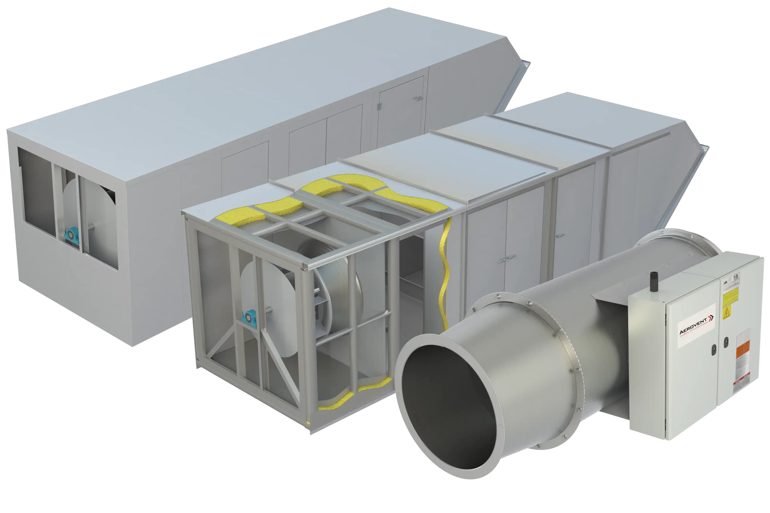
The intersection of the system curve and the fan curve is the operating point. If calculations are incorrect, the fan may operate in a “stall” region (surge) or operate inefficiently. For commercial applications requiring high volumes against moderate static pressures, a tubeaxial commercial fan belt driven unit is often specified. The belt drive allows for final RPM adjustments in the field (via sheave sizing) to dial in the exact CFM calculated in the design phase.

Engineers must also calculate Brake Horsepower (BHP) including drive losses to size the motor correctly. Undersizing a motor based on optimistic static pressure calculations will lead to thermal overload and premature failure.

Terminal Unit and Grille Sizing

The final step in the calculation chain is the delivery point. Sizing grilles and registers involves calculating Face Velocity and Throw Distance. Face velocity (FPM) is determined by CFM / Effective Area. If the velocity is too high, it generates noise (NC criteria). If too low, it fails to induce room air mixing.

Engineers must consult performance data to select a supply grille single double deflection model that provides the correct “throw”—the distance the air stream travels before slowing to a terminal velocity (usually 50 FPM). This calculation ensures that air reaches the occupied zone without creating drafts on the occupants.

Advanced Optimization Strategies

Demand-Controlled Ventilation (DCV) Calculations

While static calculations set the baseline, modern efficiency demands dynamic control. Demand-Controlled Ventilation (DCV) utilizes CO2 sensors to estimate real-time population Pz. Instead of ventilating for the design population (peak), the system modulates outdoor air based on actual occupancy.

The calculation logic involves resetting the outdoor air damper position based on a PID loop maintaining indoor CO2 levels typically 700 PPM above outdoor levels. This optimization is where the hidden value of calculation lies: by mathematically proving that low-occupancy periods require less ventilation, engineers can reduce the thermal load on the chiller and boiler significantly, leading to massive operational savings.

Building Envelope Leakage Adjustments

Ventilation calculations often assume a sealed box, but buildings leak. Engineers must account for infiltration and exfiltration. By calculating the building envelope tightness (often derived from blower door tests), engineers can adjust the supply/return offset. To maintain positive building pressure (preventing unfiltered outdoor air from entering), the Supply CFM is typically calculated to be 5% to 10% higher than the Return/Exhaust CFM total.

Selecting Efficient Duct Types

Optimization also extends to material selection. The roughness factor (ε) of the duct material affects the friction calculation. Lined ducts have higher roughness than bare metal. Flexible ducts have significantly higher pressure drops than rigid ducts. Knowing how to select the best HVAC ventilation duct types involves calculating the lifecycle energy cost of the fan overcoming resistance versus the upfront installation cost. Often, upsizing a duct by just two inches dramatically reduces pressure drop (and fan energy) due to the inverse square law of velocity.

Practical Step-by-Step Calculation Scenario

Defining the Hypothetical Space

To synthesize these concepts, consider a medium commercial office space. The parameters are as follows:

• Room Dimensions: 50 ft x 50 ft (2,500 sq. ft.)
• Ceiling Height: 10 ft
• Occupancy: 15 people (Average density office work).
• Sensible Heat Load: Calculated at 30,000 BTU/hr.
• Supply Air Temperature: 55°F.
• Room Design Temperature: 75°F.

Executing the Math: From CFM to Duct Sizing

Step 1: Calculate Thermal CFM
Using the sensible heat formula: CFM = 30,000 / (1.08 x (75 - 55)).
CFM = 30,000 / (1.08 x 20)
CFM = 30,000 / 21.6
Result: 1,388 CFM required for cooling.

Step 2: Calculate Ventilation Requirements (ASHRAE 62.1)
Assume Rp = 5 CFM/person and Ra = 0.06 CFM/sq.ft.
Vbz = (5 x 15) + (0.06 x 2,500)
Vbz = 75 + 150 = 225 CFM of outdoor air required.

Step 3: System Selection
Since the thermal CFM (1,388) is greater than the ventilation CFM (225), the fan must be sized for 1,388 CFM. The system will be set to bring in 225 CFM of fresh air (approx. 16% OA) and recirculate the rest.

Step 4: Duct Sizing
Targeting a friction rate of 0.1″ wg/100ft. Using a ductulator or calculation tool:
For 1,388 CFM, a round spiral duct would need to be approximately 14 inches in diameter (Velocity ~1,300 FPM). If using rectangular duct, a 12″ x 14″ duct would result in similar velocity and pressure drop characteristics. This confirms the importance of precise math in translating load to physical infrastructure.

The Intersection of Physics and Performance

Mastering HVAC ventilation calculation is the definitive line between a system that merely functions and one that performs with optimal efficiency. As we have explored, the journey from theoretical physics to practical application involves a rigorous understanding of fluid dynamics, thermodynamics, and regulatory compliance. The formulas for CFM, ACH, and friction loss are not just abstract mathematical exercises; they are the blueprints for occupant health, structural integrity, and long-term energy sustainability.

From Formula to Fabrication

The transition from a calculation on a spreadsheet to physical installation is where engineering precision is tested. The data derived from your load calculations dictates every hardware decision you make. It determines whether a standard fan is sufficient or if the static pressure requirements demand a robust tubeaxial commercial fan belt driven unit to overcome system resistance. Without accurate math, equipment is often oversized “just to be safe,” leading to short-cycling, humidity issues, and inflated operational costs.

The Critical Role of Ductwork Selection

Perhaps nowhere is the impact of calculation more visible than in the infrastructure of the building. Understanding how to size air ducts is essential for maintaining the velocity and pressure balance established in your design phase. The choice of material impacts the friction rate, which in turn alters the fan energy required. While rectangular duct and fittings may offer advantages in tight ceiling plenums, the calculations often favor the aerodynamic superiority of spiral duct and fittings for high-velocity applications. Every elbow, transition, and linear foot of ductwork must be accounted for to ensure the air reaches the terminal units as intended.

Balancing Compliance with Comfort

While adhering to ASHRAE Standard 62.1 provides a legal safety net, true engineering excellence strives for more than just the minimum. A comprehensive understanding of what is ventilation in HVAC reveals that it is a dual mandate: diluting contaminants while maintaining thermal comfort. By integrating occupancy diversity factors and zone effectiveness metrics, engineers can design systems that respond dynamically to real-world conditions rather than static hypothetical peaks.

This balance extends to the final delivery of air. The calculations for throw and face velocity ensure that the selected supply grille single double deflection models distribute air effectively without creating drafts or noise. It is the final step in a chain of custody that begins with a BTU calculation and ends with a comfortable occupant.

The Financial Impact of Precision

Ultimately, the value of rigorous calculation lies in the Return on Investment (ROI). Systems designed with precise attention to sensible and latent heat loads, psychrometrics, and static pressure physics consume less energy and last longer. By avoiding the pitfalls of undersized air ducts or mismatched fans, building owners avoid the compounding costs of retrofits and high utility bills. Advanced strategies like Demand-Controlled Ventilation further prove that mathematics is the most powerful tool for energy conservation available to the modern engineer.

Conclusion

In the complex world of HVAC design, calculation is the compass that guides every decision. From the initial assessment of sensible and latent loads to the selection of the final diffuser, every step relies on the immutable laws of physics. By mastering these formulas and understanding how to apply them to hardware selection—whether it be fans, ducts, or control systems—you ensure that your projects meet the highest standards of safety, efficiency, and comfort.

The future of ventilation belongs to those who can bridge the gap between theoretical data and practical application. As technology evolves and buildings become tighter and more efficient, the margin for error shrinks. Rely on precise calculations, adhere to industry standards, and select high-quality components to build systems that stand the test of time. Your commitment to accuracy today defines the building performance of tomorrow.